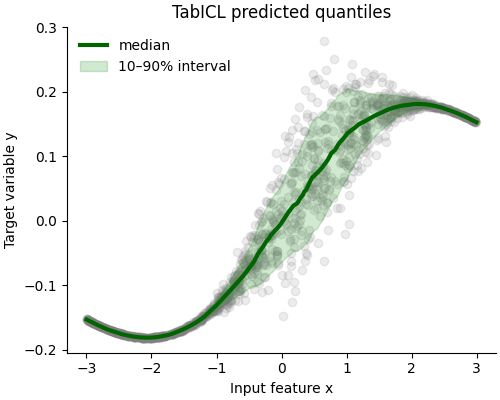
Quantile regression with TabICL

This example shows the TabICL predicted quantiles on a simple 1D regression problem with heteroscedastic noise.

import numpy as np
from scipy.special import expit
import matplotlib.pyplot as plt
from sklearn.model_selection import train_test_split
from scipy.stats import norm
from tabicl import TabICLRegressor

Generate heteroscedastic data

We first generate a simple one-dimensional regression task to illustrate the natural ability of TabICL to model predictive uncertainty in the presence of heteroscedastic noise.

Heteroscedasticity means that the variance of the target random variable y is not constant over the feature space: there are regions of x for which y is much harder to predict than for other.

The following data generating process is heteroscedastic because true_y_std is not constant: it is defined as a function of x.

rng = np.random.default_rng(0)
n_samples = int(3e3)
x = rng.uniform(low=-3, high=3, size=n_samples)
X = x.reshape((n_samples, 1))


def true_y_mean(x):
    return expit(x) - 0.5 - 0.1 * x


def true_y_std(x):
    return 0.07 * np.exp(-((x - 0.5) ** 2) / 0.9)


y = rng.normal(loc=true_y_mean(x), scale=true_y_std(x))

X_train, X_test, y_train, y_test = train_test_split(
    X, y, test_size=1 / 2, random_state=0
)

Fit TabICL and estimate quantiles

The TabICL model is fitted with n_estimators=1 to disable ensembling to speed-up the execution (at the cost of slightly worse predictions).

The model then estimates quantiles of the distribution of Y|X for each test data point. If the model is good, we expect 80% of the observed values of y to lie between the predicted lower (0.1) and upper (0.9) quantile values.

The 0.5 quantile prediction estimates the median of Y|X: we expect 50% of the observation to lie above and the remaining 50% to lie below.

tabicl = TabICLRegressor(n_estimators=1)
tabicl.fit(X_train, y_train)

alphas = [0.10, 0.5, 0.90]
quantiles = tabicl.predict(X_test, output_type="quantiles", alphas=alphas)

Plot the quantiles predicted by TabICL

The predictions of the lower and upper quantiles are sorted by increasing value of x to define the boarder of a shaded area that represents the predictive uncertainty of the model on this dataset. We can observe that the (vertical) width of the prediction interval is much larger for x values between -0.5 and 1.5 than elsewhere and naturally adapts to the noise level of y given x.

For x values below -1. or above 2., the TabICL model is very confident (narrow prediction intervals): indeed we can observe that y is nearly a deterministic (noise free) function of x in those regions.

def plot_data_and_quantiles(X_test, y_test, quantiles):

    _, ax = plt.subplots(figsize=(5, 4), constrained_layout=True)

    # Plot test data points
    ax.scatter(
        x=X_test,
        y=y_test,
        alpha=0.15,
        color="gray"
    )

    # sort test points for a clean line plot (optional)
    order = np.argsort(X_test[:, 0])
    x_sorted = X_test[order, 0]

    # Plot median
    ax.plot(x_sorted, quantiles[order, 1],
            color='darkgreen', lw=3, label="median")

    # Plot 10-90% interval
    ax.fill_between(x_sorted, quantiles[order, 0],
                    quantiles[order, 2], alpha=0.18,
                    color="green", label="10–90% interval")

    ax.legend(frameon=False)
    ax.set(xlabel="Input feature x", ylabel="Target variable y")
    ax.spines[['top', 'right']].set_visible(False)
    ax.set_title("TabICL predicted quantiles")


plot_data_and_quantiles(X_test, y_test, quantiles)