Model interpretability with TabICL

TabICL comes with a fast approximations of SHAP values. It is much faster than using black-box shape routines on TabICL which is slow.

Here we demo it on dataset on wages

The dataset: wages

from sklearn.datasets import fetch_openml

survey = fetch_openml(data_id=534, as_frame=True)

X = survey.data[survey.feature_names]

A quick glance at the data with skrub’s TableReport

import skrub

skrub.TableReport(X)

Please enable javascript

The skrub table reports need javascript to display correctly. If you are displaying a report in a Jupyter notebook and you see this message, you may need to re-execute the cell or to trust the notebook (button on the top right or "File > Trust notebook").

We need to convert the categorical features to numeric ones. We can do this with pandas’ get_dummies

import pandas as pd

X = pd.get_dummies(X, drop_first=True)

The values to predict: wages

y = survey.target.values.ravel()

Split out a test set

from sklearn.model_selection import train_test_split

X_train, X_test, y_train, y_test = train_test_split(X, y)

Our TabICL model

from tabicl import TabICLRegressor

clf = TabICLRegressor(n_estimators=4, device="cpu")
clf.fit(X_train, y_train)

Checkpoint 'tabicl-regressor-v2-20260212.ckpt' not cached.
 Downloading from Hugging Face Hub (jingang/TabICL).

TabICLRegressor(device='cpu', n_estimators=4)

In a Jupyter environment, please rerun this cell to show the HTML representation or trust the notebook.
On GitHub, the HTML representation is unable to render, please try loading this page with nbviewer.org.

Shap-like interpretability

Use TabICL’s fast approximations of shap-like values and plot them

This part of the example requires to install the shap extra: pip install ‘tabicl[shap]

from tabicl.shap import get_shap_values, plot_shap

# Compute the shap values
sv = get_shap_values(clf, X_test[:10])

PermutationExplainer explainer:  10%|█         | 1/10 [00:00<?, ?it/s]
PermutationExplainer explainer:  30%|███       | 3/10 [01:39<02:44, 23.52s/it]
PermutationExplainer explainer:  40%|████      | 4/10 [02:26<03:18, 33.15s/it]
PermutationExplainer explainer:  50%|█████     | 5/10 [03:12<03:10, 38.15s/it]
PermutationExplainer explainer:  60%|██████    | 6/10 [03:59<02:44, 41.09s/it]
PermutationExplainer explainer:  70%|███████   | 7/10 [04:45<02:08, 42.89s/it]
PermutationExplainer explainer:  80%|████████  | 8/10 [05:32<01:28, 44.08s/it]
PermutationExplainer explainer:  90%|█████████ | 9/10 [06:19<00:44, 44.88s/it]
PermutationExplainer explainer: 100%|██████████| 10/10 [07:05<00:00, 45.39s/it]
PermutationExplainer explainer: 11it [07:52, 45.97s/it]
PermutationExplainer explainer: 11it [07:52, 47.29s/it]

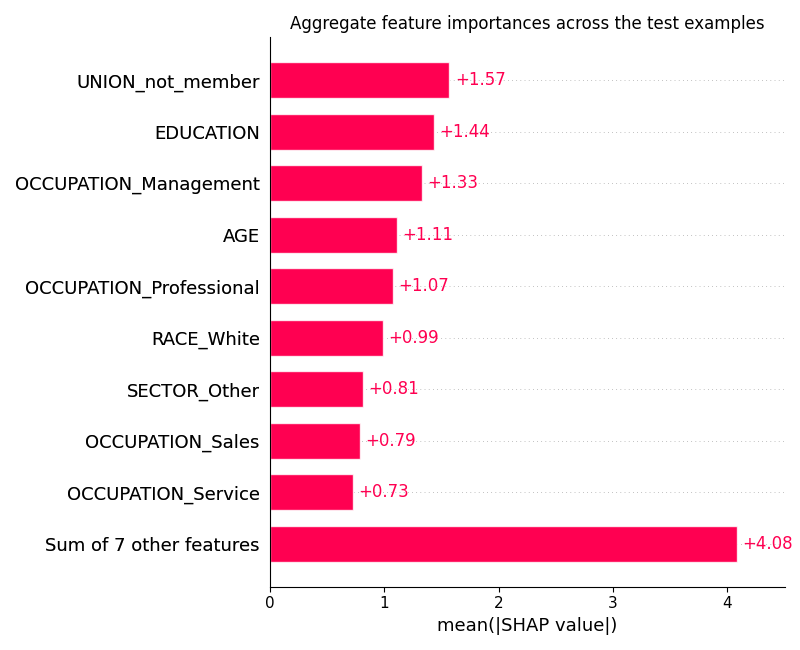
Bar plot of mean absolute SHAP values, showing aggregate feature importances

plot_shap(sv, kind="bar")

Beeswarm plot showing per-sample SHAP values for each feature

plot_shap(sv, kind="beeswarm")

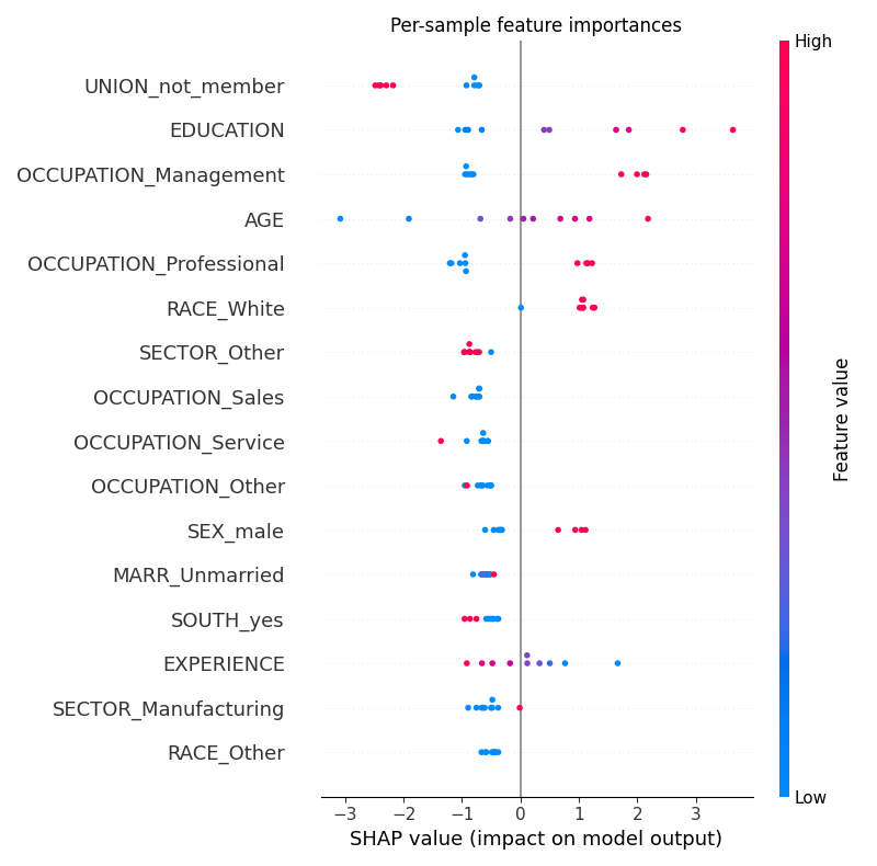
Note that these are approximate SHAP values, and not exact ones.