Note
Go to the end to download the full example code.
Fine-tuning TabICL for classification#
Adapt a pretrained TabICL classifier to a single dataset with
tabicl.FinetunedTabICLClassifier (cross-entropy on raw logits,
same objective the pretrained head was fit with).
Note
A CUDA GPU is recommended for large-scale fine-tuning. Multi-GPU via
torchrun --nproc-per-node=N (auto-detected).
import os

import matplotlib.pyplot as plt
import numpy as np
from sklearn.metrics import accuracy_score, log_loss, roc_auc_score
from sklearn.model_selection import train_test_split

from tabicl import FinetunedTabICLClassifier, TabICLClassifier
Target: one moderate feature (curved split), one hard feature (disc)#
ISLAND_CENTER = np.array([-1.5, 0.5], dtype=np.float32)
ISLAND_RADIUS = 0.9
MAIN_AMP = 0.7  # sine amplitude of the main boundary
MAIN_FREQ = 1.2  # sine frequency of the main boundary


def target_fn(X: np.ndarray) -> np.ndarray:
    y = (X[:, 0] + MAIN_AMP * np.sin(MAIN_FREQ * X[:, 1]) > 0).astype(np.int64)
    inside = np.sum((X - ISLAND_CENTER) ** 2, axis=1) < ISLAND_RADIUS**2
    return np.where(inside, 1, y)


def make_dataset(n_samples: int = 1_500, random_state: int = 0):
    rng = np.random.RandomState(random_state)
    X = rng.uniform(-3.0, 3.0, size=(n_samples, 2)).astype(np.float32)
    y = target_fn(X)
    return X, y


X, y = make_dataset(n_samples=1_500, random_state=0)

# Split: 80 train (sparse at the disc) / 200 val (early stopping) / rest test.
# Stratify on the joint (class, inside-disc) key so the training set
# reliably captures ~5 disc points.
in_island_all = np.sum((X - ISLAND_CENTER) ** 2, axis=1) < ISLAND_RADIUS**2
strat_key = y.astype(int) * 2 + in_island_all.astype(int)

X_train, X_rest, y_train, y_rest, _, strat_rest = train_test_split(
    X, y, strat_key, train_size=80, random_state=0, stratify=strat_key
)
X_val, X_test, y_val, y_test = train_test_split(X_rest, y_rest, train_size=200, random_state=0, stratify=strat_rest)

is_main_process = int(os.environ.get("LOCAL_RANK", "0")) == 0


def _metrics(proba: np.ndarray, y_true: np.ndarray) -> tuple[float, float, float]:
    preds = np.argmax(proba, axis=1)
    return (
        float(roc_auc_score(y_true, proba[:, 1])),
        float(log_loss(y_true, proba, labels=[0, 1])),
        float(accuracy_score(y_true, preds)),
    )
Baseline — zero-shot TabICL#
Expected: draws the vertical split, smears the island.
base = TabICLClassifier(n_estimators=4, random_state=0)
base.fit(X_train, y_train)
base_proba = base.predict_proba(X_test)
base_auc, base_ll, base_acc = _metrics(base_proba, y_test)
# Captured for the training-curve reference line in Figure 2.
base_val_auc = float(roc_auc_score(y_val, base.predict_proba(X_val)[:, 1]))
Fine-tune#
_HistoryLogger below is installed via the same
_make_experiment_logger hook wandb_kwargs uses, to capture per-epoch
val metrics for Figure 2 without pulling in W&B.
history: dict[str, list[float]] = {
    "epoch": [],
    "val_roc_auc": [],
    "val_log_loss": [],
    "val_accuracy": [],
    "train_loss": [],
}


class _HistoryLogger:
    """Record per-epoch validation metrics into ``history``."""

    def setup(self, config):
        del config

    def log_step(self, metrics, step):
        del metrics, step

    def log_epoch(self, metrics, step):
        del step
        history["epoch"].append(int(metrics.get("train/epoch", len(history["epoch"]))) + 1)
        history["val_roc_auc"].append(float(metrics.get("val/roc_auc", np.nan)))
        history["val_log_loss"].append(float(metrics.get("val/log_loss", np.nan)))
        history["val_accuracy"].append(float(metrics.get("val/accuracy", np.nan)))
        history["train_loss"].append(float(metrics.get("train/mean_loss", np.nan)))

    def finish(self):
        pass


clf = FinetunedTabICLClassifier(
    epochs=60,
    learning_rate=1e-5,
    n_estimators_finetune=2,
    n_estimators_validation=2,
    n_estimators_inference=4,
    early_stopping=True,
    patience=10,
    eval_metric="roc_auc",
    random_state=0,
    verbose=True,
)
clf._make_experiment_logger = lambda: _HistoryLogger()
clf.fit(X_train, y_train, X_val=X_val, y_val=y_val)
/home/docs/checkouts/readthedocs.org/user_builds/tabicl/checkouts/latest/tutorials/finetune_classifier.py:136: UserWarning: `output_dir` is not set; no checkpoints will be saved and all fine-tuning progress is lost if the run is interrupted.
  clf.fit(X_train, y_train, X_val=X_val, y_val=y_val)
Baseline val roc_auc: 0.9811

Fine-tune:   0%|          | 0/60 [00:00<?, ?it/s]
Fine-tune:   0%|          | 0/60 [00:01<?, ?it/s, train_loss=0.2665, val_roc_auc=0.9811, best=0.9811, s/epoch=0.7]
Fine-tune:   2%|▏         | 1/60 [00:01<01:08,  1.17s/it, train_loss=0.2665, val_roc_auc=0.9811, best=0.9811, s/epoch=0.7]
Fine-tune:   2%|▏         | 1/60 [00:02<01:08,  1.17s/it, train_loss=0.1482, val_roc_auc=0.9806, best=0.9811, s/epoch=0.6]
Fine-tune:   3%|▎         | 2/60 [00:02<01:06,  1.15s/it, train_loss=0.1482, val_roc_auc=0.9806, best=0.9811, s/epoch=0.6]
Fine-tune:   3%|▎         | 2/60 [00:03<01:06,  1.15s/it, train_loss=0.0947, val_roc_auc=0.9815, best=0.9815, s/epoch=0.6]
Fine-tune:   5%|▌         | 3/60 [00:03<01:05,  1.16s/it, train_loss=0.0947, val_roc_auc=0.9815, best=0.9815, s/epoch=0.6]
Fine-tune:   5%|▌         | 3/60 [00:04<01:05,  1.16s/it, train_loss=0.1667, val_roc_auc=0.9835, best=0.9835, s/epoch=0.6]
Fine-tune:   7%|▋         | 4/60 [00:04<01:04,  1.15s/it, train_loss=0.1667, val_roc_auc=0.9835, best=0.9835, s/epoch=0.6]
Fine-tune:   7%|▋         | 4/60 [00:05<01:04,  1.15s/it, train_loss=0.7136, val_roc_auc=0.9857, best=0.9857, s/epoch=0.6]
Fine-tune:   8%|▊         | 5/60 [00:05<01:02,  1.14s/it, train_loss=0.7136, val_roc_auc=0.9857, best=0.9857, s/epoch=0.6]
Fine-tune:   8%|▊         | 5/60 [00:06<01:02,  1.14s/it, train_loss=0.6135, val_roc_auc=0.9892, best=0.9892, s/epoch=0.6]
Fine-tune:  10%|█         | 6/60 [00:06<01:01,  1.14s/it, train_loss=0.6135, val_roc_auc=0.9892, best=0.9892, s/epoch=0.6]
Fine-tune:  10%|█         | 6/60 [00:07<01:01,  1.14s/it, train_loss=0.0148, val_roc_auc=0.9911, best=0.9911, s/epoch=0.6]
Fine-tune:  12%|█▏        | 7/60 [00:07<01:00,  1.13s/it, train_loss=0.0148, val_roc_auc=0.9911, best=0.9911, s/epoch=0.6]
Fine-tune:  12%|█▏        | 7/60 [00:09<01:00,  1.13s/it, train_loss=0.0391, val_roc_auc=0.9916, best=0.9916, s/epoch=0.6]
Fine-tune:  13%|█▎        | 8/60 [00:09<00:58,  1.13s/it, train_loss=0.0391, val_roc_auc=0.9916, best=0.9916, s/epoch=0.6]
Fine-tune:  13%|█▎        | 8/60 [00:10<00:58,  1.13s/it, train_loss=0.0748, val_roc_auc=0.9921, best=0.9921, s/epoch=0.6]
Fine-tune:  15%|█▌        | 9/60 [00:10<00:57,  1.13s/it, train_loss=0.0748, val_roc_auc=0.9921, best=0.9921, s/epoch=0.6]
Fine-tune:  15%|█▌        | 9/60 [00:11<00:57,  1.13s/it, train_loss=0.2246, val_roc_auc=0.9922, best=0.9922, s/epoch=0.6]
Fine-tune:  17%|█▋        | 10/60 [00:11<00:56,  1.13s/it, train_loss=0.2246, val_roc_auc=0.9922, best=0.9922, s/epoch=0.6]
Fine-tune:  17%|█▋        | 10/60 [00:12<00:56,  1.13s/it, train_loss=0.2194, val_roc_auc=0.9924, best=0.9924, s/epoch=0.6]
Fine-tune:  18%|█▊        | 11/60 [00:12<00:55,  1.12s/it, train_loss=0.2194, val_roc_auc=0.9924, best=0.9924, s/epoch=0.6]
Fine-tune:  18%|█▊        | 11/60 [00:13<00:55,  1.12s/it, train_loss=0.1049, val_roc_auc=0.9920, best=0.9924, s/epoch=0.6]
Fine-tune:  20%|██        | 12/60 [00:13<00:53,  1.12s/it, train_loss=0.1049, val_roc_auc=0.9920, best=0.9924, s/epoch=0.6]
Fine-tune:  20%|██        | 12/60 [00:14<00:53,  1.12s/it, train_loss=0.0780, val_roc_auc=0.9921, best=0.9924, s/epoch=0.6]
Fine-tune:  22%|██▏       | 13/60 [00:14<00:52,  1.11s/it, train_loss=0.0780, val_roc_auc=0.9921, best=0.9924, s/epoch=0.6]
Fine-tune:  22%|██▏       | 13/60 [00:15<00:52,  1.11s/it, train_loss=0.1736, val_roc_auc=0.9925, best=0.9925, s/epoch=0.6]
Fine-tune:  23%|██▎       | 14/60 [00:15<00:51,  1.11s/it, train_loss=0.1736, val_roc_auc=0.9925, best=0.9925, s/epoch=0.6]
Fine-tune:  23%|██▎       | 14/60 [00:16<00:51,  1.11s/it, train_loss=0.2008, val_roc_auc=0.9922, best=0.9925, s/epoch=0.6]
Fine-tune:  25%|██▌       | 15/60 [00:16<00:49,  1.11s/it, train_loss=0.2008, val_roc_auc=0.9922, best=0.9925, s/epoch=0.6]
Fine-tune:  25%|██▌       | 15/60 [00:18<00:49,  1.11s/it, train_loss=0.2372, val_roc_auc=0.9920, best=0.9925, s/epoch=0.6]
Fine-tune:  27%|██▋       | 16/60 [00:18<00:48,  1.11s/it, train_loss=0.2372, val_roc_auc=0.9920, best=0.9925, s/epoch=0.6]
Fine-tune:  27%|██▋       | 16/60 [00:19<00:48,  1.11s/it, train_loss=0.1123, val_roc_auc=0.9919, best=0.9925, s/epoch=0.6]
Fine-tune:  28%|██▊       | 17/60 [00:19<00:47,  1.11s/it, train_loss=0.1123, val_roc_auc=0.9919, best=0.9925, s/epoch=0.6]
Fine-tune:  28%|██▊       | 17/60 [00:20<00:47,  1.11s/it, train_loss=0.2490, val_roc_auc=0.9920, best=0.9925, s/epoch=0.6]
Fine-tune:  30%|███       | 18/60 [00:20<00:46,  1.11s/it, train_loss=0.2490, val_roc_auc=0.9920, best=0.9925, s/epoch=0.6]
Fine-tune:  30%|███       | 18/60 [00:21<00:46,  1.11s/it, train_loss=0.0581, val_roc_auc=0.9924, best=0.9925, s/epoch=0.6]
Fine-tune:  32%|███▏      | 19/60 [00:21<00:45,  1.11s/it, train_loss=0.0581, val_roc_auc=0.9924, best=0.9925, s/epoch=0.6]
Fine-tune:  32%|███▏      | 19/60 [00:22<00:45,  1.11s/it, train_loss=0.1895, val_roc_auc=0.9924, best=0.9925, s/epoch=0.6]
Fine-tune:  33%|███▎      | 20/60 [00:22<00:44,  1.10s/it, train_loss=0.1895, val_roc_auc=0.9924, best=0.9925, s/epoch=0.6]
Fine-tune:  33%|███▎      | 20/60 [00:23<00:44,  1.10s/it, train_loss=0.0116, val_roc_auc=0.9924, best=0.9925, s/epoch=0.6]
Fine-tune:  35%|███▌      | 21/60 [00:23<00:43,  1.10s/it, train_loss=0.0116, val_roc_auc=0.9924, best=0.9925, s/epoch=0.6]
Fine-tune:  35%|███▌      | 21/60 [00:24<00:43,  1.10s/it, train_loss=0.2290, val_roc_auc=0.9919, best=0.9925, s/epoch=0.6]
Fine-tune:  37%|███▋      | 22/60 [00:24<00:41,  1.10s/it, train_loss=0.2290, val_roc_auc=0.9919, best=0.9925, s/epoch=0.6]
Fine-tune:  37%|███▋      | 22/60 [00:25<00:41,  1.10s/it, train_loss=0.1353, val_roc_auc=0.9917, best=0.9925, s/epoch=0.6]
Fine-tune:  38%|███▊      | 23/60 [00:25<00:40,  1.10s/it, train_loss=0.1353, val_roc_auc=0.9917, best=0.9925, s/epoch=0.6]
Fine-tune:  38%|███▊      | 23/60 [00:26<00:40,  1.10s/it, train_loss=0.1583, val_roc_auc=0.9915, best=0.9925, s/epoch=0.6]
Fine-tune:  38%|███▊      | 23/60 [00:26<00:43,  1.17s/it, train_loss=0.1583, val_roc_auc=0.9915, best=0.9925, s/epoch=0.6]
Evaluate on the held-out test set#
ft_proba = clf.predict_proba(X_test)
ft_auc, ft_ll, ft_acc = _metrics(ft_proba, y_test)

if is_main_process:
    header = f"{'metric':<12}{'pretrained':>14}{'fine-tuned':>14}{'Δ':>14}"
    rule = "=" * len(header)
    print()
    print(rule)
    print(f"Test-set metrics  (n_train={len(X_train)}, n_test={len(X_test)})")
    print(rule)
    print(header)
    print("-" * len(header))
    print(f"{'ROC-AUC ↑':<12}{base_auc:>14.4f}{ft_auc:>14.4f}{ft_auc - base_auc:>+14.4f}")
    print(f"{'log-loss ↓':<12}{base_ll:>14.4f}{ft_ll:>14.4f}{ft_ll - base_ll:>+14.4f}")
    print(f"{'accuracy ↑':<12}{base_acc:>14.4f}{ft_acc:>14.4f}{ft_acc - base_acc:>+14.4f}")
    print(rule)
======================================================
Test-set metrics  (n_train=80, n_test=1220)
======================================================
metric          pretrained    fine-tuned             Δ
------------------------------------------------------
ROC-AUC ↑           0.9790        0.9898       +0.0109
log-loss ↓          0.1880        0.1278       -0.0602
accuracy ↑          0.9057        0.9393       +0.0336
======================================================
Figure 1 — Decision boundaries + probability contours#
Dashed black curve = true main boundary. Dashed yellow ring = true disc boundary. Panel titles split accuracy into inside-disc vs outside-disc so the localized improvement is visible at a glance.
if is_main_process:
    h = 0.15
    xx, yy = np.meshgrid(
        np.arange(-3.0, 3.0 + h, h),
        np.arange(-3.0, 3.0 + h, h),
    )
    grid = np.c_[xx.ravel(), yy.ravel()].astype(np.float32)
    p_base = base.predict_proba(grid)[:, 1].reshape(xx.shape)
    p_ft = clf.predict_proba(grid)[:, 1].reshape(xx.shape)

    base_pred = np.argmax(base_proba, axis=1)
    ft_pred = np.argmax(ft_proba, axis=1)
    in_island_test = np.sum((X_test - ISLAND_CENTER) ** 2, axis=1) < ISLAND_RADIUS**2

    # Precompute the true main boundary curve x₁ = −MAIN_AMP·sin(MAIN_FREQ·x₂)
    x2_curve = np.linspace(-3.0, 3.0, 400)
    x1_curve = -MAIN_AMP * np.sin(MAIN_FREQ * x2_curve)

    fig1, axes = plt.subplots(1, 2, figsize=(12.0, 5.4), sharex=True, sharey=True, constrained_layout=True)
    cf = None
    # Consistent emerald for every "ground truth" reference so they read
    # as a group, distinct from the solid-black model decision contour.
    TRUTH_COLOR = "#10b981"
    for ax, title, grid_p, preds, (auc, acc) in [
        (axes[0], "Pretrained TabICL", p_base, base_pred, (base_auc, base_acc)),
        (axes[1], "Fine-tuned TabICL", p_ft, ft_pred, (ft_auc, ft_acc)),
    ]:
        cf = ax.contourf(xx, yy, grid_p, levels=20, cmap="RdYlBu_r", alpha=0.85, vmin=0.0, vmax=1.0)
        # 0.5 decision contour, heavy black — the model's own boundary.
        ax.contour(xx, yy, grid_p, levels=[0.5], colors="black", linewidths=2.0)
        # True main boundary (sine curve) — dashed reference, shared across
        # panels so the comparison with the model boundary is direct.
        ax.plot(x1_curve, x2_curve, color=TRUTH_COLOR, lw=2.0, ls="--", label="true main boundary")
        # True disc boundary — both panels share this reference too.
        theta = np.linspace(0, 2 * np.pi, 200)
        ax.plot(
            ISLAND_CENTER[0] + ISLAND_RADIUS * np.cos(theta),
            ISLAND_CENTER[1] + ISLAND_RADIUS * np.sin(theta),
            color=TRUTH_COLOR,
            lw=2.4,
            ls="--",
            label="true disc boundary",
        )
        # Training data (shape-coded by true label).
        m0 = y_train == 0
        m1 = y_train == 1
        ax.scatter(
            X_train[m0, 0],
            X_train[m0, 1],
            marker="o",
            c="#1d4ed8",
            s=46,
            edgecolor="white",
            linewidths=1.0,
            label="train y=0",
        )
        ax.scatter(
            X_train[m1, 0],
            X_train[m1, 1],
            marker="s",
            c="#b91c1c",
            s=46,
            edgecolor="white",
            linewidths=1.0,
            label="train y=1",
        )
        # Split test-set accuracy into "inside the disc" vs "outside"
        # to quantify the localized improvement directly in the title.
        acc_in = (
            float((preds[in_island_test] == y_test[in_island_test]).mean()) if in_island_test.any() else float("nan")
        )
        acc_out = (
            float((preds[~in_island_test] == y_test[~in_island_test]).mean())
            if (~in_island_test).any()
            else float("nan")
        )
        ax.set_title(f"{title}\nROC-AUC={auc:.3f}  acc={acc:.3f}", fontsize=12)
        ax.set_xlabel("x₁", fontsize=11)
        ax.set_xlim(-3, 3)
        ax.set_ylim(-3, 3)
        ax.tick_params(labelsize=10)
        ax.grid(alpha=0.25)
    axes[0].set_ylabel("x₂", fontsize=11)
    axes[0].legend(loc="lower right", framealpha=0.92, fontsize=9)
    cbar = fig1.colorbar(cf, ax=axes, shrink=0.85)
    cbar.set_label("P(class 1)", fontsize=11)
    cbar.ax.tick_params(labelsize=9)
    fig1.suptitle("Decision boundaries: pretrained vs. fine-tuned", fontsize=14)
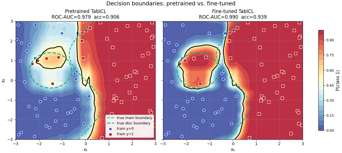
Figure 2 — Training dynamics + metric comparison#
Left: val ROC-AUC per epoch; dashed line = pretrained floor, star = best epoch kept by the safety net. Right: test-set ROC-AUC / log-loss / accuracy bars.
if is_main_process and history["epoch"]:
    fig2, (ax_tr, ax_bar) = plt.subplots(1, 2, figsize=(12.8, 4.8), constrained_layout=True)

    ep = history["epoch"]
    val_auc = history["val_roc_auc"]
    ax_tr.plot(ep, val_auc, "o-", color="#0f766e", lw=2.0, markersize=5, label="fine-tuning: val ROC-AUC")
    ax_tr.axhline(
        base_val_auc,
        ls="--",
        color="#64748b",
        lw=1.5,
        label=f"pretrained baseline ({base_val_auc:.3f})",
    )
    best_idx = int(np.nanargmax(val_auc))
    ax_tr.scatter(
        [ep[best_idx]],
        [val_auc[best_idx]],
        marker="*",
        s=220,
        color="#f59e0b",
        edgecolor="black",
        linewidths=0.8,
        zorder=5,
        label=f"best epoch ({val_auc[best_idx]:.3f} @ epoch {ep[best_idx]})",
    )
    ax_tr.set_xlabel("epoch")
    ax_tr.set_ylabel("validation ROC-AUC (higher is better)")
    ax_tr.set_title("Validation metric across fine-tuning epochs")
    ax_tr.grid(alpha=0.3)
    ax_tr.legend(fontsize=9, loc="lower right")

    metric_names = ["ROC-AUC ↑", "log-loss ↓", "accuracy ↑"]
    base_vals = [base_auc, base_ll, base_acc]
    ft_vals = [ft_auc, ft_ll, ft_acc]
    x_pos = np.arange(len(metric_names))
    w = 0.38
    bars_b = ax_bar.bar(x_pos - w / 2, base_vals, w, color="#64748b", label="pretrained")
    bars_f = ax_bar.bar(x_pos + w / 2, ft_vals, w, color="#0f766e", label="fine-tuned")
    for bars, vals in [(bars_b, base_vals), (bars_f, ft_vals)]:
        for rect, v in zip(bars, vals):
            y_anchor = v + (0.02 if v >= 0 else -0.04)
            ax_bar.text(
                rect.get_x() + rect.get_width() / 2,
                y_anchor,
                f"{v:.3f}",
                ha="center",
                va="bottom" if v >= 0 else "top",
                fontsize=8,
            )
    ax_bar.set_xticks(x_pos)
    ax_bar.set_xticklabels(metric_names)
    ax_bar.set_title("Test-set metrics: pretrained vs. fine-tuned")
    ax_bar.set_ylabel("metric value")
    ax_bar.axhline(0, color="black", lw=0.5)
    ax_bar.grid(alpha=0.25, axis="y")
    ax_bar.legend(fontsize=9, loc="upper right")

    fig2.suptitle("Training dynamics & test-set gains", fontsize=13)
    plt.show()

Total running time of the script: (0 minutes 46.800 seconds)