Time series forecasting

This tutorial shows how to do zero-shot univariate forecasting with tabicl.TabICLForecaster. Make sure the forecast dependencies are installed:

pip install tabicl[forecast]

Time series forecasting as tabular regression

tabicl.TabICLForecaster is inspired by TabPFN-TS.

The forecaster wraps tabicl.TabICLRegressor and turns forecasting into a tabular regression problem:

• each row is one timestamp,

• the target column is the series value,

• time-aware features are added automatically (index, calendar, seasonality).

Note

Compared with tabicl.TabICLClassifier and tabicl.TabICLRegressor, the forecasting interface is newer and has not yet been evaluated on a large public benchmark. We may later provide evaluations and enhancements for time series forecasting.

import numpy as np
import pandas as pd
from tabicl import TabICLForecaster
from tabicl.forecast import plot_forecast

Build a synthetic univariate series

We create a daily series that mixes a linear trend, a weekly seasonality, an annual seasonality, and Gaussian noise.

This makes the task intuitive: the model should extrapolate trend and recurring patterns into the future.

rng = np.random.default_rng(0)
n_timesteps = 365 * 2  # two years of daily observations
dates = pd.date_range(start="2022-01-01", periods=n_timesteps, freq="D")
t = np.arange(n_timesteps)

trend = 0.05 * t
weekly_season = 5.0 * np.sin(2 * np.pi * t / 7)
annual_season = 10.0 * np.sin(2 * np.pi * t / 365)
noise = rng.normal(scale=1.5, size=n_timesteps)

target = trend + weekly_season + annual_season + noise

# For a single time series, ``timestamp`` and ``target`` are sufficient.
df = pd.DataFrame({"timestamp": dates, "target": target})
df.head()

	timestamp	target
0	2022-01-01	0.188595
1	2022-01-02	3.933134
2	2022-01-03	6.279490
3	2022-01-04	2.992966
4	2022-01-05	-2.084898

This DataFrame follows the input format required by tabicl.TabICLForecaster.predict_df():

• required columns: timestamp, target

• optional column: item_id (for multiple series)

• use prediction_length for regular horizons, or future_df when you already know future timestamps/covariates

Define forecast horizon and hold-out period

We keep the last prediction_length points as a pseudo-future set.

• context_df is the observed history provided to the forecaster.

• test_df is only used for visual comparison.

prediction_length = 30
context_df = df.iloc[:-prediction_length]
test_df = df.iloc[-prediction_length:]

Forecast with TabICLForecaster

tabicl.TabICLForecaster.predict_df() returns one row per future timestamp, with a point forecast and quantile columns for uncertainty.

forecaster = TabICLForecaster()
pred_df = forecaster.predict_df(context_df, prediction_length=prediction_length)

Predicting time series:   0%|          | 0/1 [00:00<?, ?it/s]
Predicting time series: 100%|██████████| 1/1 [00:05<00:00,  5.89s/it]
Predicting time series: 100%|██████████| 1/1 [00:05<00:00,  5.89s/it]

Plot context, forecast, and held-out truth

fig, axes = plot_forecast(context_df=context_df, pred_df=pred_df, test_df=test_df)

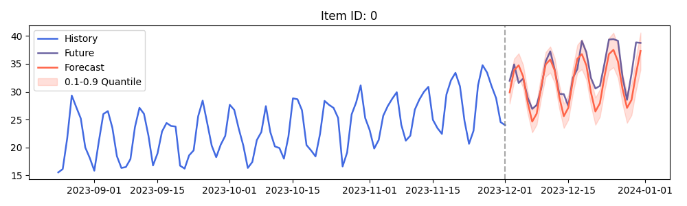
A good forecast should continue the upward trend and recover the recurring seasonal pattern visible in the held-out future values, which the TabICLForecaster does successfully in this example.